
Advent of R Functions
Explore 15 essential pieces of R code to streamline your data analysis and visualization workflow. From creating directories and handling files to customizing ggplot and working with logit scales, these snippets can help you enhance your programming efficiency and maintain cleaner scripts.
It is advent! And we all know by now how much I LOVE advent and Christmas. Keeping true to who I am and that I finally have some extra energy for things like this, this advent brings you a series of 24 pieces of code I often use in my work, and that I hope can be of interest and help to you.
1st of December - Creating a directory
I often find myself doing quite some file handling in my work, often leading to many of the same things happening over and over in slightly different contexts. If you try to create files in a directory that does not exists, R will throw an error
penguins <- palmerpenguins::penguins
write.table(penguins, "new_folder/penguins.csv")
## Warning in file(file, ifelse(append, "a", "w")): cannot open file 'new_folder/
## penguins.csv': No such file or directory
## Error in file(file, ifelse(append, "a", "w")): cannot open the connection
So, I very often have this piece of code in any file-writing function I make to create the folder. But R will also throw annoying warnings if the folder already exists, which I also don’t like.
dir.create("new_folder") # no warning
dir.create("new_folder") # produces warning
## Warning in dir.create("new_folder"): 'new_folder' already exists
The solution, is to check if the directory already exists, and make it if it does not.
if(!dir.exists("new_folder")) dir.create("new_folder")
Actually, I often end up using a little convenience function for this, since I do it quite often.
dir_create <- function(x, ...){
  if(!dir.exists(x))
    dir.create(x, recursive = TRUE, ...)
}
dir_create("new_folder")
dir_create("new_folder")
Here, I can have a function to easily create new folders, with any extra arguments to dir.create passed along using the ... (ellipsis), and only make the directory if it does not already exist.
This is a staple bit of code for me.
Hope it will help you get your scripts tidier!
2nd of December - Writing subsetted data to files
I’ll continue in the same line as the first day, with working with the file system. I’ve shown how I create a utility function to create new directories if they don’t exist, and now we want to write files to them!
I’ll continue using base-R, as for this first part of the calendar, I am emulating work I do on our offline server where I often struggle with getting dependencies installed in stable ways.
We have our lovely penguins data set, and I want to save one file per penguin species in the data.table. That is, I want to split the data.frame into three data.frames each containing only the data from a single penguin species. Then I want to save each of those to file.
First we need to split the data set.
Usually, when not on the server, I’d do some {dplyr} nest_by magic, but I cannot in this case.
So we need to deal with what we have.
Neatly, base-R has the split function, which does exactly what I want.
penguins |>
  split(~species)
## $Adelie
## # A tibble: 152 × 8
## species island bill_length_mm bill_depth_mm flipper_…¹ body_…² sex year
## <fct> <fct> <dbl> <dbl> <int> <int> <fct> <int>
## 1 Adelie Torgersen 39.1 18.7 181 3750 male 2007
## 2 Adelie Torgersen 39.5 17.4 186 3800 fema… 2007
## 3 Adelie Torgersen 40.3 18 195 3250 fema… 2007
## 4 Adelie Torgersen NA NA NA NA <NA> 2007
## 5 Adelie Torgersen 36.7 19.3 193 3450 fema… 2007
## 6 Adelie Torgersen 39.3 20.6 190 3650 male 2007
## 7 Adelie Torgersen 38.9 17.8 181 3625 fema… 2007
## 8 Adelie Torgersen 39.2 19.6 195 4675 male 2007
## 9 Adelie Torgersen 34.1 18.1 193 3475 <NA> 2007
## 10 Adelie Torgersen 42 20.2 190 4250 <NA> 2007
## # … with 142 more rows, and abbreviated variable names ¹flipper_length_mm,
## # ²body_mass_g
##
## $Chinstrap
## # A tibble: 68 × 8
## species island bill_length_mm bill_depth_mm flipper_l…¹ body_…² sex year
## <fct> <fct> <dbl> <dbl> <int> <int> <fct> <int>
## 1 Chinstrap Dream 46.5 17.9 192 3500 fema… 2007
## 2 Chinstrap Dream 50 19.5 196 3900 male 2007
## 3 Chinstrap Dream 51.3 19.2 193 3650 male 2007
## 4 Chinstrap Dream 45.4 18.7 188 3525 fema… 2007
## 5 Chinstrap Dream 52.7 19.8 197 3725 male 2007
## 6 Chinstrap Dream 45.2 17.8 198 3950 fema… 2007
## 7 Chinstrap Dream 46.1 18.2 178 3250 fema… 2007
## 8 Chinstrap Dream 51.3 18.2 197 3750 male 2007
## 9 Chinstrap Dream 46 18.9 195 4150 fema… 2007
## 10 Chinstrap Dream 51.3 19.9 198 3700 male 2007
## # … with 58 more rows, and abbreviated variable names ¹flipper_length_mm,
## # ²body_mass_g
##
## $Gentoo
## # A tibble: 124 × 8
## species island bill_length_mm bill_depth_mm flipper_len…¹ body_…² sex year
## <fct> <fct> <dbl> <dbl> <int> <int> <fct> <int>
## 1 Gentoo Biscoe 46.1 13.2 211 4500 fema… 2007
## 2 Gentoo Biscoe 50 16.3 230 5700 male 2007
## 3 Gentoo Biscoe 48.7 14.1 210 4450 fema… 2007
## 4 Gentoo Biscoe 50 15.2 218 5700 male 2007
## 5 Gentoo Biscoe 47.6 14.5 215 5400 male 2007
## 6 Gentoo Biscoe 46.5 13.5 210 4550 fema… 2007
## 7 Gentoo Biscoe 45.4 14.6 211 4800 fema… 2007
## 8 Gentoo Biscoe 46.7 15.3 219 5200 male 2007
## 9 Gentoo Biscoe 43.3 13.4 209 4400 fema… 2007
## 10 Gentoo Biscoe 46.8 15.4 215 5150 male 2007
## # … with 114 more rows, and abbreviated variable names ¹flipper_length_mm,
## # ²body_mass_g
Out comes three data.frames with each data set in them, preserved in a list. Awesome!
Then, I need to save them to files.
I will use lapply (list apply) to loop through the list, and save each file.
I send each data set into the lapply function, giving them the placeholder name x.
So, x will be one data.frame.
Then I write the csv to file, using the species name.
penguins |>
  split(~species) |>
  lapply(function(x){
    write.csv(x, paste0(unique(x$species), ".csv"), row.names = FALSE)
  })
## $Adelie
## NULL
##
## $Chinstrap
## NULL
##
## $Gentoo
## NULL
list.files(".", "csv")
## [1] "Adelie.csv" "Chinstrap.csv" "csvs" "Gentoo.csv"
Ok. so the files are there, but I am not super happy with this. I don’t like capitalisation in my file names, and they are not in a folder. I also cannot easily change the grouping factor, if I for instance wanted to save by island or sex in stead. To do that, I’ll construct a function that will do my work for me in a standardised way. It’s going to be quite a doozy, but its such a convenient thing for me!
save_files <- function(data, group, directory) {
  # get column name from formula
  colname <- as.character(group)[-1]

  # Create directory
  dir <- file.path(directory, colname)
  dir_create(dir)

  # split the data
  tmp <- split(data, group)

  # internal file name constructor
  .filename <- function(data){
    # get unique value, make lower, append .csv
    g <- unique(data[[colname]]) |>
      tolower() |>
      paste0(".csv")
    # construct file path with directory, grouping and dataset
    file.path(dir, g)
  }

  # apply file names to the split data
  # makes `sapply` give a really nice output
  names(tmp) <- sapply(tmp, .filename)

  # write the filees!
  sapply(tmp, function(x) {
    write.csv(x,
              .filename(x),
              row.names = FALSE)
  })
}
save_files(penguins, ~species, "csvs")
## $`csvs/species/adelie.csv`
## NULL
##
## $`csvs/species/chinstrap.csv`
## NULL
##
## $`csvs/species/gentoo.csv`
## NULL
save_files(penguins, ~island, "csvs")
## $`csvs/island/biscoe.csv`
## NULL
##
## $`csvs/island/dream.csv`
## NULL
##
## $`csvs/island/torgersen.csv`
## NULL
list.files("csvs", recursive = TRUE)
## [1] "island/biscoe.csv"     "island/dream.csv"      "island/torgersen.csv"
## [4] "species/adelie.csv"    "species/chinstrap.csv" "species/gentoo.csv"
See? Now we have everything I wanted. The files are all in neatly ordered folders, named neatly, and it just makes my organisatory heart happy! Admittedly, it is kind of a large function, but it is also very convenient for quite some stuff I do. For instance, while I regularly run analyses on complete datasets, some times I need to get some things done in subgroups of the data to inspect possible origins of effects that can be hard when I look at the entire data as a whole. And many of the analyses I run are heavy computing, so I need to prepare files to send analyses to a computing cluster.
This tidbit of code is nice to have to create these datafiles I need.
3rd of December - Reading in lots of files
Now that we have managed to create lots of files, based on data groupings, let us also see how we can read them in efficiently. I’ve made so many absolutely horrid pipelines to do this, before I figured out this way of doing it.
The pre-requisites for this is that all the files you are reading in all have the same columns, if they don’t, the last bit will fail.
# list all files in the species folder,
# contiaing the ending "csv" and
# keep the entire relative path.
list.files("csvs/species", "csv$", full.names = TRUE)
## [1] "csvs/species/adelie.csv"    "csvs/species/chinstrap.csv"
## [3] "csvs/species/gentoo.csv"
We have three files, and we want to read the all in, at once and get them into a list.
We’ve worked with lapply() before, and we will again here.
We will use the list of file paths in lapply, and run the read.csv function on them all.
This should give us a list of three data sets.
list.files("csvs/species", "csv$", full.names = TRUE) |>
  lapply(read.csv)
## [[1]]
##   species    island bill_length_mm bill_depth_mm flipper_length_mm body_mass_g
## 1  Adelie Torgersen           39.1          18.7               181        3750
## 2  Adelie Torgersen           39.5          17.4               186        3800
## 3  Adelie Torgersen           40.3          18.0               195        3250
##      sex year
## 1   male 2007
## 2 female 2007
## 3 female 2007
##  [ reached 'max' / getOption("max.print") -- omitted 149 rows ]
##
## [[2]]
##     species island bill_length_mm bill_depth_mm flipper_length_mm body_mass_g
## 1 Chinstrap  Dream           46.5          17.9               192        3500
## 2 Chinstrap  Dream           50.0          19.5               196        3900
## 3 Chinstrap  Dream           51.3          19.2               193        3650
##      sex year
## 1 female 2007
## 2   male 2007
## 3   male 2007
##  [ reached 'max' / getOption("max.print") -- omitted 65 rows ]
##
## [[3]]
##   species island bill_length_mm bill_depth_mm flipper_length_mm body_mass_g
## 1  Gentoo Biscoe           46.1          13.2               211        4500
## 2  Gentoo Biscoe           50.0          16.3               230        5700
## 3  Gentoo Biscoe           48.7          14.1               210        4450
##      sex year
## 1 female 2007
## 2   male 2007
## 3 female 2007
##  [ reached 'max' / getOption("max.print") -- omitted 121 rows ]
Once that is done, we also want to have them all combined into a single data set, i.e. back to our full penguins data set.
To do that, we will use do.call and rbind to achieve this.
Now, do.call is a bit of magic, and I am not entirely sure of what it does in all contexts.
In this context, it will run through the list, and run rbind on each data set, so that we get a single one out.
data_list <- list.files("csvs/species", "csv$", full.names = TRUE) |>
  lapply(read.csv)

do.call(rbind, data_list)
##   species    island bill_length_mm bill_depth_mm flipper_length_mm body_mass_g
## 1  Adelie Torgersen           39.1          18.7               181        3750
## 2  Adelie Torgersen           39.5          17.4               186        3800
## 3  Adelie Torgersen           40.3          18.0               195        3250
##      sex year
## 1   male 2007
## 2 female 2007
## 3 female 2007
##  [ reached 'max' / getOption("max.print") -- omitted 341 rows ]
And now we have our data frame with 344 rows back! But! Usually, I would want to know which file each row comes from. In the penguins data here, that is not a huge issue, as the species column basically already tells us that. But there might be lots of other reasons you’d like to know, for instance for debugging the original data (in case there are suspicious entries), or because the source file information is not inherent in the data. To do that, we need a little custom function.
merge_files <- function(path, pattern, func = read.csv, ...){
  file_list <- list.files(path, pattern, full.names = TRUE)
  data_list <- lapply(file_list, func, ...)
  # loop through data_list length
  # apply new column with source information
  data_list <- lapply(seq_along(data_list), function(x){
    data_list[[x]]$src <- file_list[x]
    data_list[[x]]
  })
  do.call(rbind, data_list)
}
merged <- merge_files("csvs/species/", "csv")
merged[, c(1:3, 9)]
##   species    island bill_length_mm                      src
## 1  Adelie Torgersen           39.1 csvs/species//adelie.csv
## 2  Adelie Torgersen           39.5 csvs/species//adelie.csv
## 3  Adelie Torgersen           40.3 csvs/species//adelie.csv
## 4  Adelie Torgersen             NA csvs/species//adelie.csv
## 5  Adelie Torgersen           36.7 csvs/species//adelie.csv
## 6  Adelie Torgersen           39.3 csvs/species//adelie.csv
## 7  Adelie Torgersen           38.9 csvs/species//adelie.csv
##  [ reached 'max' / getOption("max.print") -- omitted 337 rows ]
Now we have it all!
The function does quite a lot, in little space, but it also allows quite some customisation.
Like, we can our selves define which read function to use, in case the data has a different delimiter than csv, and we can also add any other named argument to that function in our main function call.
4th of December - fixing column names
I love the janitor package. It has some cleaning functions for data that just make my world so much easier. And while janitor’s dependencies are small enough that I can often get it when I need, I still have install issues in certain cases. In those cases, I need to do some simple steps to improve my data dealings.
Depending on how bad things are, there are some small things we can to to help with column naming. I’m being a little cheeky an borrowing the example data from janitor. I will not be able to make it as neat as janitor, but we can make it much better!
test_df <- as.data.frame(matrix(ncol = 6, nrow = 5))
names(test_df) <- c("firstName", "ábc@!*", "% successful (2009)",
                    "REPEAT VALUE", "REPEAT VALUE", "")

# add some data
test_df[1, ] <- c("jane", "JANE", TRUE, NA, 10, NA)
test_df[2, ] <- c("elleven", "011", FALSE, NA, NA, NA)
test_df[3, ] <- c("Henry", "001", NA, NA, 20, NA)
test_df
##   firstName ábc@!* % successful (2009) REPEAT VALUE REPEAT VALUE
## 1      jane   JANE                TRUE         <NA>           10 <NA>
## 2   elleven    011               FALSE         <NA>         <NA> <NA>
## 3     Henry    001                <NA>         <NA>           20 <NA>
## 4      <NA>   <NA>                <NA>         <NA>         <NA> <NA>
## 5      <NA>   <NA>                <NA>         <NA>         <NA> <NA>
I think we can all agree this is no fun column names to deal with! Keeping to base R and some regular expression (oh man, I need to google those expressions every time!), we can do a decent bit of cleaning.
clean_names <- function(data, col_prefix = "v"){
  colnames <- names(data)

  # turn camelCase to snake_case
  colnames <- gsub("(?![A-Z])(\\G(?!^)|\\b[a-zA-Z][a-z]*)([A-Z][a-z]*|\\d+)",
       "\\1_\\2", colnames, ignore.case = FALSE, perl = TRUE)

  # turn white space into _
  colnames <- gsub(" ", "_", colnames)

  # turn to lower case
  colnames <- tolower(colnames)

  # remove punctuations except _
  colnames <- gsub("[^a-z0-9_]+", "", colnames)

  # trim _ from beginning and end
  colnames <- gsub("^_|_$", "", colnames)

  # add column names to columns missing them
  k <- sapply(match("", colnames), function(x){
    colnames[x] <<- paste0(col_prefix, x)
  })

  # apply name changes
  names(data) <- colnames

  # returned the renamed data
  data
}
test_df <- clean_names(test_df)
test_df
##   first_name   bc successful_2009 repeat_value repeat_value   v6
## 1       jane JANE            TRUE         <NA>           10 <NA>
## 2    elleven  011           FALSE         <NA>         <NA> <NA>
## 3      Henry  001            <NA>         <NA>           20 <NA>
## 4       <NA> <NA>            <NA>         <NA>         <NA> <NA>
## 5       <NA> <NA>            <NA>         <NA>         <NA> <NA>
Ok, we get pretty close to what I was after.
camelCase turned into snake_case, all lower case, and weird punctuations removed.
We also manage to name columns without names.
What we miss is that the á in “ábc@!*” is removed.
This is because my regular expression is interpreting as a weird special character to remove.
To replace it with an a I’d need to get a library that would know how to translate it, and I don’t/can’t do that.
So, I’ll have to deal with that manually.
5th of December - removing empty columns
In the type of data I deal with, I do also quite often have to deal with columns containing no data. Either because the subsetted data are missing a variable, or because a file I read in thinks there is another column, when there truly is not. I want a nice easy way to deal with that. Again janitor would be my “online” solution, but when offline, I need to deal in my own code.
test_df
##   first_name   bc successful_2009 repeat_value repeat_value   v6
## 1       jane JANE            TRUE         <NA>           10 <NA>
## 2    elleven  011           FALSE         <NA>         <NA> <NA>
## 3      Henry  001            <NA>         <NA>           20 <NA>
## 4       <NA> <NA>            <NA>         <NA>         <NA> <NA>
## 5       <NA> <NA>            <NA>         <NA>         <NA> <NA>
We made a data.frame yesterday with missing values completely from rows 4 and 5, and partial missing data from 2 and 3, while row 1 is the only complete row of data. And in columns 4 and 6 we are completely missing any data. We want a simple way to remove all columns that have no information, so we have something simpler to work with.
na_rm_col <- function(data){
  # find columns with only missing values
  idx <- apply(data, 2, function(x) all(is.na(x)))

  # keep only columns where there is data
  data[, !idx]
}
test_df <- na_rm_col(test_df)
test_df
##   first_name   bc successful_2009 repeat_value
## 1       jane JANE            TRUE           10
## 2    elleven  011           FALSE         <NA>
## 3      Henry  001            <NA>           20
## 4       <NA> <NA>            <NA>         <NA>
## 5       <NA> <NA>            <NA>         <NA>
With this function we first apply across the columns (apply dimension 2) and check if all values are NA.
If they are, we make sure we don’t return a data.frame with those columns.
The function is neither long nor particularly complicated (though apply does take a little time to get the hang of), and its super quick!
6th of December - removing empty rows
Yesterday we removed empty columns, but we might also need to remove empty rows! Imagine having subsetted columns, and now, lots of your rows actually don’t contain meaningful information any more. No use in having them around, lets just get rid of them!
The code is remarkably similar to yesterdays code,
na_rm_row <- function(data){
  # find columns with only missing values
  idx <- apply(data, 1, function(x) all(is.na(x)))

  # keep only rows where there is data
  data[!idx, ]
}
test_df2 <- na_rm_row(test_df)
test_df2
##   first_name   bc successful_2009 repeat_value
## 1       jane JANE            TRUE           10
## 2    elleven  011           FALSE         <NA>
## 3      Henry  001            <NA>           20
We are still using apply, but this time along the 1 dimension, which is rows.
And we are using the exact same function inside apply!
Then, we subset the rows with the inverse of that output, giving us only the rows we want.
7th of December - removing empty rows 2nd ed.
In our last post, we removed rows that had all NA values, but this is often not the case.
Likely, you’ll have some identifier columns that are always populated, and you’ll want to make sure you check for NA not in those columns.
I.e. we want to discard rows where certain columns only have NA not necessarily all!
This one becomes a little trickier!
na_rm_row <- function(data,
                      col_names = names(data),
                      col_inverse = FALSE){
  # Get column index for wanted cols
  col_idx <- names(data) %in% col_names

  # Get column names by index
  cols <-  names(data)[col_idx]

  # Reverse if you want exclude the columns
  if(col_inverse){
    cols <- names(data)[!col_idx]
  }

  # subset the data
  # force output to data.frame
  tmp <- data.frame(data[, cols])

  # find rows with only missing values
  idx <- apply(tmp, 1, function(x) all(is.na(x)))

  # keep only rows where there is data
  data[!idx, ]
}
na_rm_row(test_df,
          col_names = c("successful_2009",
                        "repeat_value"))
##   first_name   bc successful_2009 repeat_value
## 1       jane JANE            TRUE           10
## 2    elleven  011           FALSE         <NA>
## 3      Henry  001            <NA>           20
na_rm_row(test_df,
          col_names = c("first_name", "bc"),
          col_inverse = TRUE)
##   first_name   bc successful_2009 repeat_value
## 1       jane JANE            TRUE           10
## 2    elleven  011           FALSE         <NA>
## 3      Henry  001            <NA>           20
So this function is a little busy.
Hopefully the code comments help understanding of what is going on.
I’ve added to option to either name columns you want to check for NAs in, or columns you want excluded from that check.
This way, we can hopefully make it work in any of the circumstances we meet.
8th of December - File extension changes
In many cases, I will read in files in one format, but want to save them - with the same file name - in another format. I prefer working with tab-separated files, as in Norway the comma is actually used for a decimal separator and we always seem to end up with issues using either comma or semi-colon separated files. So, I might read in a file, do some cleaning, and then want to save it to file just with another extension name. In my case, I usually opt for changing “csv” to “tsv” to make it clear that the file is tab-separated.
So, we need to use the file name, strip the extension and add our own. We have saved our penguin data as csv, so lets read them in, and then save them as tsv.
# Find all files ending with csv in a folder
files <- list.files("csvs/species", "csv", full.names = TRUE)
files
## [1] "csvs/species/adelie.csv"    "csvs/species/chinstrap.csv"
## [3] "csvs/species/gentoo.csv"
# read in the files
dt_list <- lapply(files, read.csv)
names(dt_list) <- files
dt_list
## $`csvs/species/adelie.csv`
##   species    island bill_length_mm bill_depth_mm flipper_length_mm body_mass_g
## 1  Adelie Torgersen           39.1          18.7               181        3750
## 2  Adelie Torgersen           39.5          17.4               186        3800
## 3  Adelie Torgersen           40.3          18.0               195        3250
##      sex year
## 1   male 2007
## 2 female 2007
## 3 female 2007
##  [ reached 'max' / getOption("max.print") -- omitted 149 rows ]
##
## $`csvs/species/chinstrap.csv`
##     species island bill_length_mm bill_depth_mm flipper_length_mm body_mass_g
## 1 Chinstrap  Dream           46.5          17.9               192        3500
## 2 Chinstrap  Dream           50.0          19.5               196        3900
## 3 Chinstrap  Dream           51.3          19.2               193        3650
##      sex year
## 1 female 2007
## 2   male 2007
## 3   male 2007
##  [ reached 'max' / getOption("max.print") -- omitted 65 rows ]
##
## $`csvs/species/gentoo.csv`
##   species island bill_length_mm bill_depth_mm flipper_length_mm body_mass_g
## 1  Gentoo Biscoe           46.1          13.2               211        4500
## 2  Gentoo Biscoe           50.0          16.3               230        5700
## 3  Gentoo Biscoe           48.7          14.1               210        4450
##      sex year
## 1 female 2007
## 2   male 2007
## 3 female 2007
##  [ reached 'max' / getOption("max.print") -- omitted 121 rows ]
csv2tsv <- function(data, file){
  # remove csv extension from file name
  file <- tools::file_path_sans_ext(file)

  # add `.tsv`
  file <- paste0(file, ".tsv")

  # print location for clarity
  cat("Saving to: ", file, "\n")

  # save it in the wanted format
  write.table(data, file,
              sep = "\t",
              row.names = FALSE,
              quote = FALSE
              )
}

# Test on one file
csv2tsv(dt_list[[1]], files[1])
## Saving to: csvs/species/adelie.tsv
That seems to work.
We first remote the file extension, then add our own .tsv to it.
Then we use the base-R table writing function, specifying exactly the format we want to save in.
I prefer not quoting strings when I’m working with tab-separated files, since people in general do not enter tabs in character vectors, so its not needed and the file content looks cleaner.
We should double check that the file looks as we intend. I’m going to use bash to do this, as its my go-to for something like this, rather than R!
head csvs/species/adelie.tsv
## species	island	bill_length_mm	bill_depth_mm	flipper_length_mm	body_mass_g	sex	year
## Adelie	Torgersen	39.1	18.7	181	3750	male	2007
## Adelie	Torgersen	39.5	17.4	186	3800	female	2007
## Adelie	Torgersen	40.3	18	195	3250	female	2007
## Adelie	Torgersen	NA	NA	NA	NA	NA	2007
## Adelie	Torgersen	36.7	19.3	193	3450	female	2007
## Adelie	Torgersen	39.3	20.6	190	3650	male	2007
## Adelie	Torgersen	38.9	17.8	181	3625	female	2007
## Adelie	Torgersen	39.2	19.6	195	4675	male	2007
## Adelie	Torgersen	34.1	18.1	193	3475	NA	2007
That looks good to me! tabs, no quotes, no row numbers.
Now we can run it on all, and I will use mapply, which makes it possible to send several vectors (of the same size) into an apply function.
mapply(
  csv2tsv,
  dt_list,
  names(dt_list)
)
## Saving to:  csvs/species/adelie.tsv
## Saving to:  csvs/species/chinstrap.tsv
## Saving to:  csvs/species/gentoo.tsv
## $`csvs/species/adelie.csv`
## NULL
##
## $`csvs/species/chinstrap.csv`
## NULL
##
## $`csvs/species/gentoo.csv`
## NULL
That seemed to work, and if we look into the species folder, we can see they are all there. csv, and tsv next to each other.
list.files("csvs/species", full.names = TRUE)
## [1] "csvs/species/adelie.csv"    "csvs/species/adelie.tsv"
## [3] "csvs/species/chinstrap.csv" "csvs/species/chinstrap.tsv"
## [5] "csvs/species/gentoo.csv"    "csvs/species/gentoo.tsv"
Now, in this case, they are the same file, just delimited differently.
Which is why I am ok with having them in the same folder (despite the parent folder being named csv).
If I have done cleaning and changed the file content in some way, I would make another folder, to clearly show the content was different, not just delimited differently.
9th of December - System commands from R
I work in neuroimaging. While most of my work now is concentrated around tabular data and software engineering, I still deal with situations where I need to call a system program from the command line, to do some stuff. Many times, I want to do some stuff and capture the result of that stuff in R. This is not always easy, depending on the complexity of what you are doing. I’ll have a small fairly “easy” example, using a command line tool that should be available to most, to just show the example.
I’ll use the command head to get the first n rows of a dataset, default is 10 rows, if we give no extra argument.
# Look at first 10 rows
system2("head", "csvs/species/adelie.tsv")
# -n [integer] gives the number of rows wanted
system2("head", "-n 5 csvs/species/adelie.tsv")

system2("head", "-n 15 csvs/species/adelie.tsv")
But the output just gets printed in the console. We want to capture it.
data <- system2("head", "-n 5 csvs/species/adelie.tsv")
data
## [1] 0
wait, what?!
Where is the data?
system2 (and system) by default does not return anything, is is a message printed to the console through something called stdout (standard out, there is also stderr, standard error).
To capture it, we need to redirect stdout, and we do this through an argument in system2.
data <- system2("head", "-n 5 csvs/species/adelie.tsv", stdout = TRUE)
data
## [1] "species\tisland\tbill_length_mm\tbill_depth_mm\tflipper_length_mm\tbody_mass_g\tsex\tyear"
## [2] "Adelie\tTorgersen\t39.1\t18.7\t181\t3750\tmale\t2007"
## [3] "Adelie\tTorgersen\t39.5\t17.4\t186\t3800\tfemale\t2007"
## [4] "Adelie\tTorgersen\t40.3\t18\t195\t3250\tfemale\t2007"
## [5] "Adelie\tTorgersen\tNA\tNA\tNA\tNA\tNA\t2007"
The data is now stored as a string vector with 15 elements. We’ll need to work with it to get it into the shape we want.
read_custom <- function(command, arguments = list()){

  # turn list of arguments into single string
  arguments <- do.call(paste, arguments)

  cat("Running:", command, arguments, sep = " ")
  # run command
  data <- system2(command, arguments, stdout = TRUE)

  # split string into elements by comma
  data <- strsplit(data, "\t")

  # bind rows together
  data <- do.call(rbind, data)

  # force into data frame
  data <- as.data.frame(data)

  # apply col names from the first row
  names(data) <- data[1, ]

  # remove first row of data, as its the col names
  data <- data[-1, ]

  # auto-detect column types
  data <- type.convert(data, as.is = TRUE)

  data
}

read_custom("head", list("-n 5", "csvs/species/adelie.tsv"))
## Running: head -n 5 csvs/species/adelie.tsv
##   species    island bill_length_mm bill_depth_mm flipper_length_mm body_mass_g
## 2  Adelie Torgersen           39.1          18.7               181        3750
## 3  Adelie Torgersen           39.5          17.4               186        3800
## 4  Adelie Torgersen           40.3          18.0               195        3250
##      sex year
## 2   male 2007
## 3 female 2007
## 4 female 2007
##  [ reached 'max' / getOption("max.print") -- omitted 1 rows ]
Now we have a custom reading in files function!
I mean, yeah read.table is hella better, but it shows what kind of amazing things you can do when need arises.
I’ve done things like this when I get very irregular files in formats that have no standard way of being read.
What is neat with this one, is that we can change the command used (as long as it does the basic same thing as head) or change the arguments quite easily.
tail for instance, is the reverse of head, giving the last rows.-
read_custom("tail", list("-n 5", "csvs/species/adelie.tsv"))
## Running: tail -n 5 csvs/species/adelie.tsv
##   Adelie Dream 36.6 18.4 184 3475 female 2009
## 2 Adelie Dream 36.0 17.8 195 3450 female 2009
## 3 Adelie Dream 37.8 18.1 193 3750   male 2009
## 4 Adelie Dream 36.0 17.1 187 3700 female 2009
##  [ reached 'max' / getOption("max.print") -- omitted 1 rows ]
Convoluted? Yes. Fun? Yes :)
10th of December - Function calling it self
Once upon a time, I made a function where I needed the function behaviour inside the function it self. It sounds weird, I know! But I was trying to get the dependency tree of packages, and I needed to get all of the dependencies and have my own function not rely on anything but base-R.
Then I learned, a function can cal it self!! That concept it still hard for me to grasp, but it does work! We just need to be very careful to have ways that the function stops calling it self when its not supposed to, else we end up in infinite loops of recursion.
# make a nested list
mock <- list(
  character = c("a", "string", "vector"),
  list = list(
    nested1 = c("nested", "list", "1"),
    nested2 = c("nested", "list", "2")
  ),
  number = 1:5
)
mock
## $character
## [1] "a"      "string" "vector"
##
## $list
## $list$nested1
## [1] "nested" "list"   "1"
##
## $list$nested2
## [1] "nested" "list"   "2"
##
##
## $number
## [1] 1 2 3 4 5
collapse_strings <- function(x){
  if(inherits(x, "list")){
    x <- sapply(x, collapse_strings)
    return(x)
  }

  # if not a character, return NULL
  if(!inherits(x, "character")){
    return(NULL)
  }

  # collapse strings else
  paste(x, collapse = " ")
}

sapply(mock, collapse_strings)
## $character
## [1] "a string vector"
##
## $list
##         nested1         nested2
## "nested list 1" "nested list 2"
##
## $number
## NULL
This function calls it self, if the vector provided is a list. This way, we know it wont be recursing into oblivion, but just if it is a list. I also added a check if the vector was not a character, as a collapse only makes sense for string vectors. Now we have a tidy function that recursively collapses string vectors.
11th of December - Empty strings to NA
I fairly often come across data that is not particularly clean. At least in terms of interfacing with the data through a computer, and let’s face it, that’s what we all mostly do :P
Often, data come in as strings when they should not, or I choose to read them in as strings to preserve data I might loose when turned into something else.
But that can also lead to some quite frustrating consequences I need to deal with, like empty cells "" or NA cells read as "NA". Le Sigh.
I have a little convenience function to deal with this situation exactly.
empty_to_na <- function(x){
  ifelse(x == "NA" | x == "" | x == "NULL",
         NA_character_,
         x)
}

c("", "Merry", "Christmas", "NA", "NULL", "!") |>
  empty_to_na()
## [1] NA "Merry" "Christmas" NA NA "!"
This is my little catch all for weird string data that I know should be NA.
After this, the remaining tedious cleaning begins, but this first step is something I use quite often to help myself.
12th of December - format for nice print
Some times, when I work in R markdown documents, I need to format numbers to look nicer. So today’s post is a short but sweet one!
thousand <- function(x){
  formatC(x,
          format = "f",
          big.mark = " ",
          digits = 0)
}
thousand(c(10000, 3000, 200, 320485))
## [1] "10 000" "3 000" "200" "320 485"
This is great for plots, but also for in-line numbers, like 102 937!
13th of December - bar chart convenience
I love me some ggplot. And most of the time, I get to use the standard build and wrap for subplots etc. But sometimes, I need some plot that is more specialised, needs som pre-computation of some sort before plotting. In those cases, I make a convenience function for the plotting, so I can call it at need, so make the same type of plot over and over for different settings.
library(ggplot2)
library(dplyr)
##
## Attaching package: 'dplyr'
## The following objects are masked from 'package:stats':
##
##     filter, lag
## The following objects are masked from 'package:base':
##
##     intersect, setdiff, setequal, union
ggbar <- function(data, grouping){

  # Must have both arguments to work
  stopifnot(!missing(data))
  stopifnot(!missing(grouping))

  # Create some summary stats
  # in this case percent
  data |>
    group_by({{grouping}}) |>
    tally() |>
    mutate(pc = n/sum(n)) |>

  # plot it!
  ggplot(aes(x = {{grouping}},
             y = n)) +
    geom_bar(aes(fill = pc),
             stat="identity",
             position = "dodge",
             colour = "darkgrey",
             linewidth = .3,
             show.legend = FALSE) +
    geom_label(aes(label = scales::percent(pc)))
}

ggbar(penguins, sex)
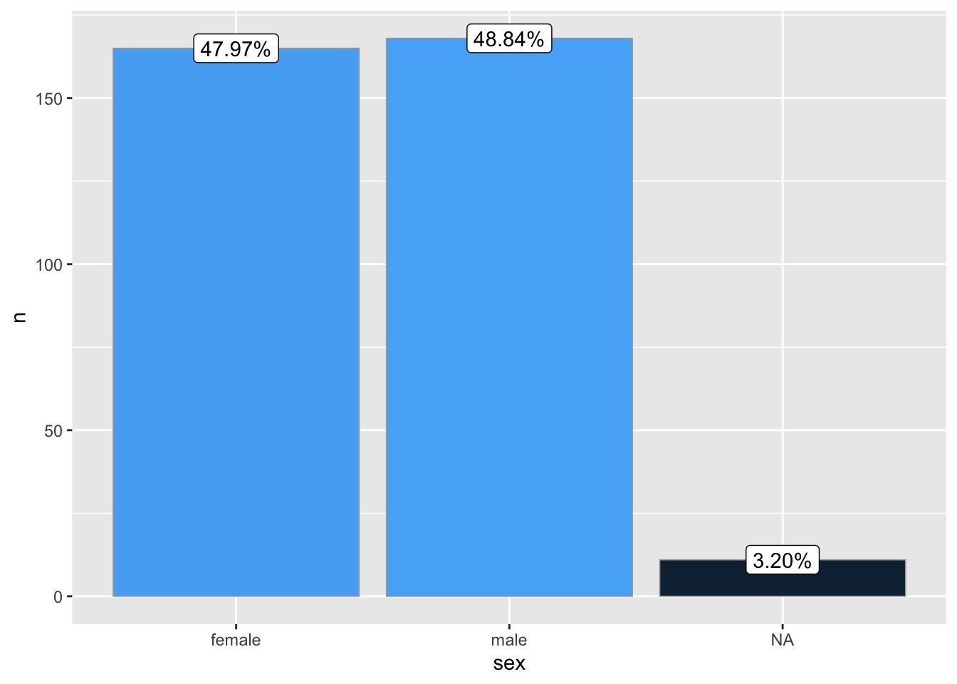
ggbar(penguins, species)
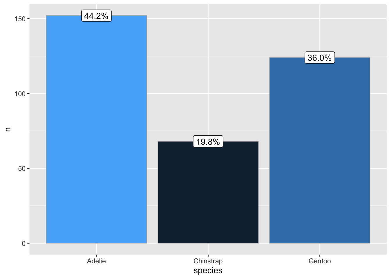
ggbar(penguins, island)
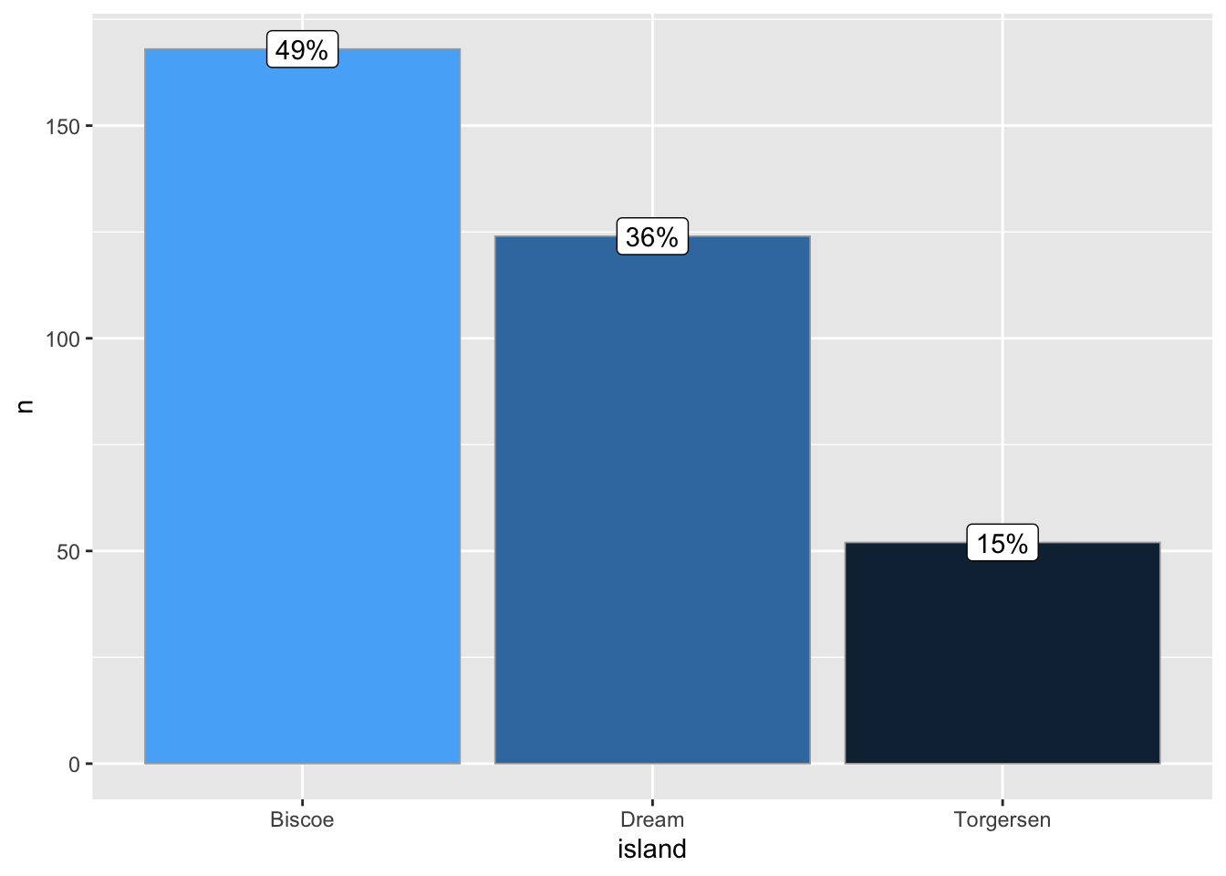
I like this a lot. It saves me a lot of copy and paste and makes everything look neat.
14th of December - wrapping plots in lists
Yesterday’s function can be used even further! Some times, it would be convenient to make subplots easily, and wrap them all together. We can do this with yesterday’s function, by adding another layer of complexity!
library(patchwork)
ggbar_wrap <- function(data, wrap, grouping){
  # Nest data by wrapping column
  nest_by(data, {{wrap}}, .key = "dt") |>
    mutate(
      # create a list of plots!
      plots = list(
             ggbar(dt,
                   grouping = {{grouping}}) +
               labs(x = "",
                    y = "",
                    subtitle = {{wrap}})
           )) |>
    pull(plots) |>

    #wrap them!
    wrap_plots(ncol = 3)
}

ggbar_wrap(penguins, species, sex)
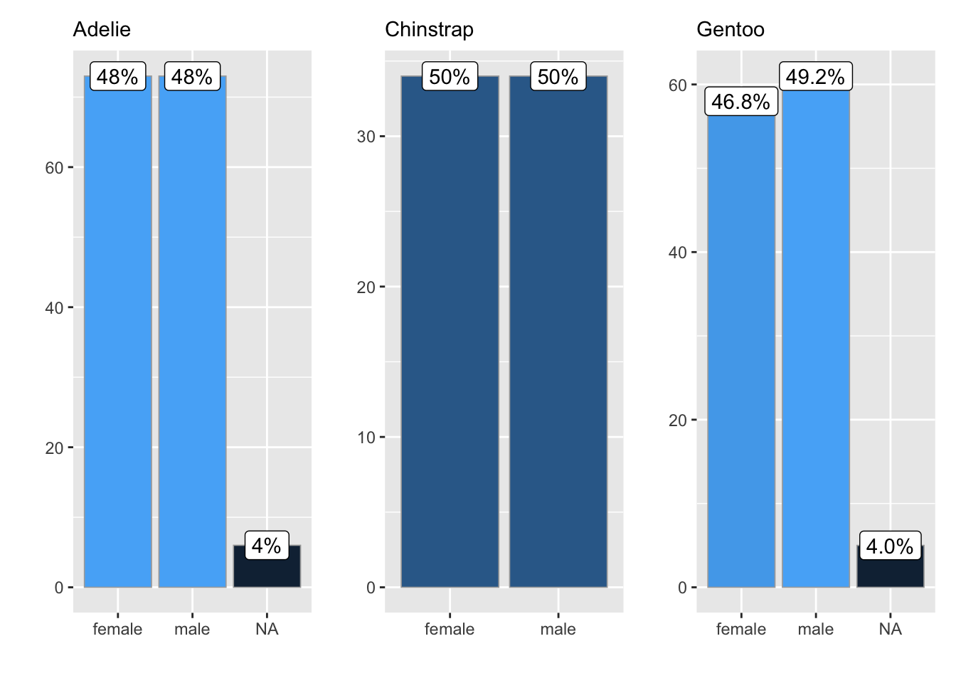
ggbar_wrap(penguins, species, island)
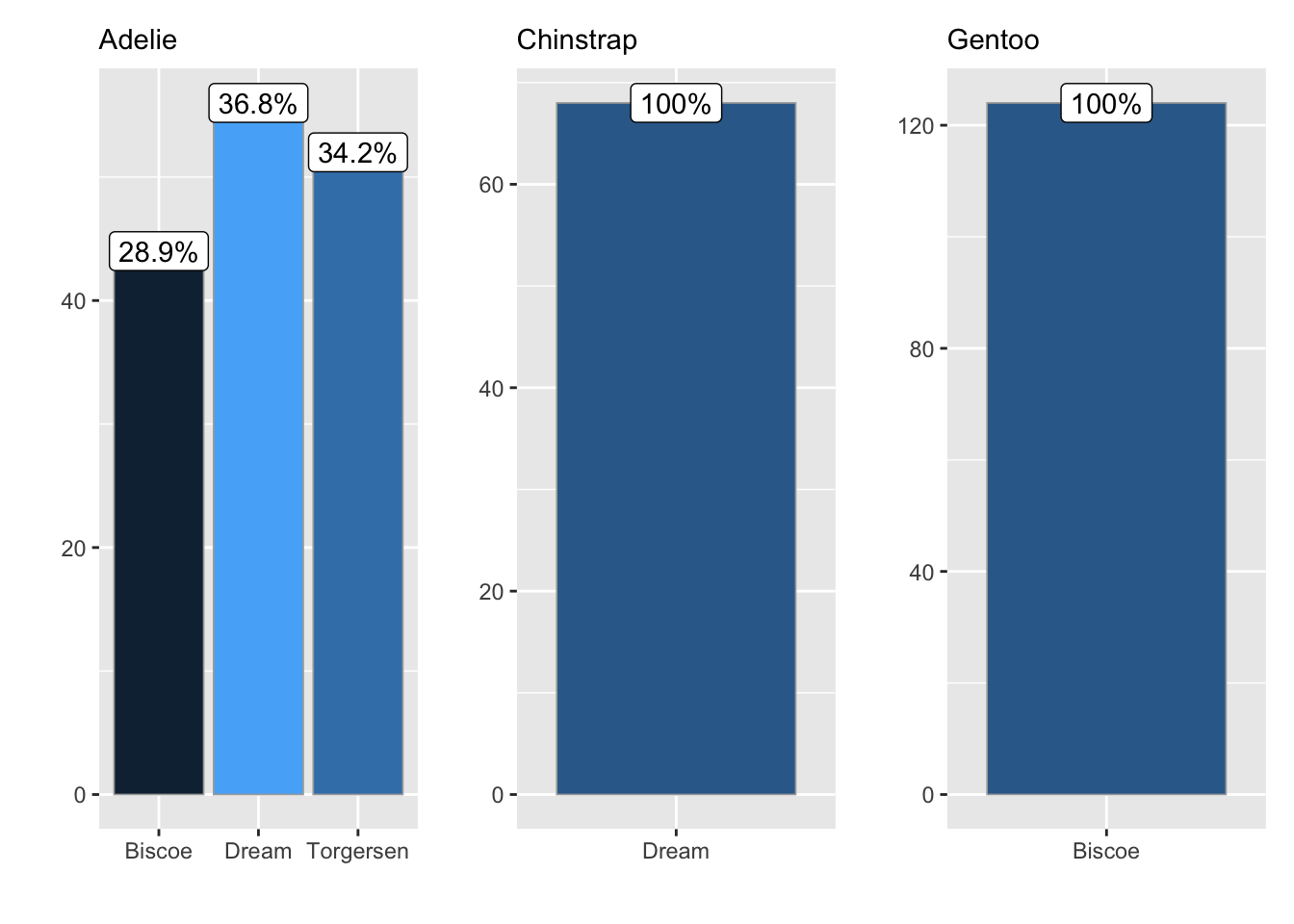
Now we can create lots of different constellations of plots!
15th of December - logit to probability
In my PhD days, I did quite some binomial modelling. That gives results in logit scale. But I struggle with logit, as they are not always the easiest to interpret, so I might want to convert them into probabilities, which my puny brain deals with a little better.
logit2prob <- function(logit){
  # turn logit into odds
  odds <- exp(logit)
  # Turn odds into probability
  odds / (1 + odds)
}
logit2prob(c(0.5, 0.3, 1.5))
## [1] 0.6224593 0.5744425 0.8175745
So, there it is. It helps me at least!!
2022-advent-of-r-functions,
author = "Dr. Mowinckel",
title = "Advent of R Functions",
url = "https://drmowinckels.io/blog/2022/advent-of-r-functions/",
year = 2022,
doi = "https://www.doi.org/10.5281/zenodo.13273527",
updated = "May 6, 2026"
}