Setting up a Freesurfer LMM through R
Learn to create model matrices for Freesurfer Linear Mixed Models (LMM) in R using built-in functions. This guide walks you through manually creating model matrices, utilizing the model.matrix function, and standardizing variables. Includes creating a function to streamline the process, making neuroimaging data analysis more efficient.
It’s been a while since I’ve been running models, I must admit. I’ve transitioned into more of a software engineering role, and I’ve been working on projects from another angle. However, I’ve been wanting to write this blogpost for a really long time. The reason for that is that I was preparing files for colleagues based on our data, to run Freesurfer Linear Mixes models, or LMM’s for short (also some times shortened to LME; Linear Mixed Effects). While I was preparing these files, I realized that there is a lot of power in R that people are not utilizing to the best extent. Me including, in the beginning!
In Neuroimaging, we are quite used to setting up model matrices (semi-) manually.
Meaning we sit down and make the matrices of 0 and 1 that
statistical models use at their core to do computations.
This is tedious and error-prone work, but we’ve become so used to it we forget to explore if there is a better way.
R, at it’s core being a statistical tool, has amazing tooling for running statistics. This tooling, includes creating model matrices for us, so we don’t have to think about it.
A simplified beginning example
The first story comes with an anecdote. My boss asked me one day to run a model for him, in R. This guy is super smart and knows exactly what he’s after. I run the model I believe he is asking for and provide the results, after which he asks me run another model to verify. In the data, we have a categorical variable, and he asks me to binarise them into variables representing each category, and use each of those in the model.
I know why he is asking for it, its what we are used to. But I also know, that is the exact model I just ran, but R does that whole binarisation (i.e. making of the model matrix) for us. Let’s first explore with mtcars, just for simplicity.
library(tidyverse)
## ── Attaching core tidyverse packages ──────────────────────── tidyverse 2.0.0 ──
## ✔ dplyr     1.1.4     ✔ readr     2.1.4
## ✔ forcats   1.0.0     ✔ stringr   1.5.1
## ✔ ggplot2   3.4.4     ✔ tibble    3.2.1
## ✔ lubridate 1.9.3     ✔ tidyr     1.3.0
## ✔ purrr     1.0.2
## ── Conflicts ────────────────────────────────────────── tidyverse_conflicts() ──
## ✖ dplyr::filter() masks stats::filter()
## ✖ dplyr::lag()    masks stats::lag()
## ℹ Use the conflicted package (<http://conflicted.r-lib.org/>) to force all conflicts to become errors
cars <- as_tibble(mtcars) |>
  mutate(
    cyl = as.factor(cyl),  # make cyl factor,
    gear = as.factor(gear),  # make gear factor
    carb = as.factor(carb),  # make carb factor
  )
cars
## # A tibble: 32 × 11
##      mpg cyl    disp    hp  drat    wt  qsec    vs    am gear  carb
##    <dbl> <fct> <dbl> <dbl> <dbl> <dbl> <dbl> <dbl> <dbl> <fct> <fct>
##  1  21   6      160    110  3.9   2.62  16.5     0     1 4     4
##  2  21   6      160    110  3.9   2.88  17.0     0     1 4     4
##  3  22.8 4      108     93  3.85  2.32  18.6     1     1 4     1
##  4  21.4 6      258    110  3.08  3.22  19.4     1     0 3     1
##  5  18.7 8      360    175  3.15  3.44  17.0     0     0 3     2
##  6  18.1 6      225    105  2.76  3.46  20.2     1     0 3     1
##  7  14.3 8      360    245  3.21  3.57  15.8     0     0 3     4
##  8  24.4 4      147.    62  3.69  3.19  20       1     0 4     2
##  9  22.8 4      141.    95  3.92  3.15  22.9     1     0 4     2
## 10  19.2 6      168.   123  3.92  3.44  18.3     1     0 4     4
## # ℹ 22 more rows
To make a point, I’ve altered some of the variables to be factors and logicals, even if in this case the numbers are scalar and meaningful.
Now, let’s say you want to know if miles per gallon (mpg) is affected by the number of cylinders (cyl), and horse powers (hp).
Your model might look like so: mpg ~ cyl + hp.
model <- lm(mpg ~ cyl + hp, data = cars)
summary(model)
##
## Call:
## lm(formula = mpg ~ cyl + hp, data = cars)
##
## Residuals:
##    Min     1Q Median     3Q    Max
## -4.818 -1.959  0.080  1.627  6.812
##
## Coefficients:
##             Estimate Std. Error t value Pr(>|t|)
## (Intercept) 28.65012    1.58779  18.044  < 2e-16 ***
## cyl6        -5.96766    1.63928  -3.640  0.00109 **
## cyl8        -8.52085    2.32607  -3.663  0.00103 **
## hp          -0.02404    0.01541  -1.560  0.12995
## ---
## Signif. codes:  0 '***' 0.001 '**' 0.01 '*' 0.05 '.' 0.1 ' ' 1
##
## Residual standard error: 3.146 on 28 degrees of freedom
## Multiple R-squared:  0.7539,	Adjusted R-squared:  0.7275
## F-statistic: 28.59 on 3 and 28 DF,  p-value: 1.14e-08
Our results lets us know that increasing from 4 cylinders to 6 and from 4 cylinders to 8 has a significant effect on miles per gallon, but increasing horse power does not.
Ok, let’s say I did this model the manual way. I’d need to binarise my categorical variables, to three columns (where 1 would indicate if the car has a specific cylinder and 0 it does not), and standardise the scalar variable (or at minimum demean it).
I could do like so:
cars_std <- cars |>
  #transmute manipulates variables, and only returns what has been manipulated
  transmute(
    mpg  = mpg,
    cyl  = cyl,
    cyl4 = ifelse(cyl == 4, 1, 0),
    cyl6 = ifelse(cyl == 6, 1, 0),
    cyl8 = ifelse(cyl == 8, 1, 0),
    hp   = hp,
    hpz  = scale(hp, center = TRUE, scale = TRUE)
  )
cars_std
## # A tibble: 32 × 7
##      mpg cyl    cyl4  cyl6  cyl8    hp hpz[,1]
##    <dbl> <fct> <dbl> <dbl> <dbl> <dbl>   <dbl>
##  1  21   6         0     1     0   110  -0.535
##  2  21   6         0     1     0   110  -0.535
##  3  22.8 4         1     0     0    93  -0.783
##  4  21.4 6         0     1     0   110  -0.535
##  5  18.7 8         0     0     1   175   0.413
##  6  18.1 6         0     1     0   105  -0.608
##  7  14.3 8         0     0     1   245   1.43
##  8  24.4 4         1     0     0    62  -1.24
##  9  22.8 4         1     0     0    95  -0.754
## 10  19.2 6         0     1     0   123  -0.345
## # ℹ 22 more rows
I’ve kept the original columns in addition to the new ones, so we can see the difference. The cylinders are now in binarised form, and the horse power is standardised.
We could now run the model like so:
model_std <- lm(mpg ~ cyl6 + cyl8 + hpz, data = cars_std)
summary(model_std)
##
## Call:
## lm(formula = mpg ~ cyl6 + cyl8 + hpz, data = cars_std)
##
## Residuals:
##    Min     1Q Median     3Q    Max
## -4.818 -1.959  0.080  1.627  6.812
##
## Coefficients:
##             Estimate Std. Error t value Pr(>|t|)
## (Intercept)   25.124      1.369  18.354  < 2e-16 ***
## cyl6          -5.968      1.639  -3.640  0.00109 **
## cyl8          -8.521      2.326  -3.663  0.00103 **
## hpz           -1.648      1.056  -1.560  0.12995
## ---
## Signif. codes:  0 '***' 0.001 '**' 0.01 '*' 0.05 '.' 0.1 ' ' 1
##
## Residual standard error: 3.146 on 28 degrees of freedom
## Multiple R-squared:  0.7539,	Adjusted R-squared:  0.7275
## F-statistic: 28.59 on 3 and 28 DF,  p-value: 1.14e-08
Notice how the results are exactly the same as the first model!
And there’s a little sneakyness here too, can you see it?
Notice how I’ve omitted the cyl4 variable in the last model, why?
Because we have a model with an intercept, and in our original model,
cyl4 is captured by the intercept, so we don’t need to include it in the model.
Indeed, we should not, as it will create issues with multicollinearity.
The intercept here means “where cyl is 4, and hp is 0”.
R’s model matrix creation
So how come this is possible? When you run a model in R, using its model formula, all the magic happens behind the scenes. When I made the variables binary and standardised, I mimmicked what R does for us. While what I did was not very complex, you can imagine that a larger model with more variables and interactions might easily start making a pretty complex model matrix. We don’t want to make that by “hand”.
How does R make the model matrix, then?
Well, the model.matrix function is what we are looking for.
It takes our formula and data, just like the lm function,
but returns something quite different.
model_matrix <- model.matrix(mpg ~ cyl + hp, data = cars)
model_matrix
##    (Intercept) cyl6 cyl8  hp
## 1            1    1    0 110
## 2            1    1    0 110
## 3            1    0    0  93
## 4            1    1    0 110
## 5            1    0    1 175
## 6            1    1    0 105
## 7            1    0    1 245
## 8            1    0    0  62
## 9            1    0    0  95
## 10           1    1    0 123
##  [ reached getOption("max.print") -- omitted 22 rows ]
## attr(,"assign")
## [1] 0 1 1 2
## attr(,"contrasts")
## attr(,"contrasts")$cyl
## [1] "contr.treatment"
This model matrix is basically what is used when running the lm model.
We do have to do some things to get what we are after, though.
We are missing mpg which is our dependent variable, we need to put that back in.
And really, if we want to use this in a Freesurfer LMM, we also need to have a column binarised for all levels of categorical variables, and demeaned for scalar variables.
So, still some work to do!
Removing the intercept
Getting rid of the intercept is, thankfully, not very difficult.
By default, all models in R have an intercept, because the models truly expand to mpg ~ 1 + cyl + hp, where + 1 is the indication to create the intercept.
If we want to remove it, we need to alter the sign of that 1 to negative: mpg ~ -1 + cyl + hp.
This means that there will be no intercept, and the model matrix will change.
model_matrix <- model.matrix(mpg ~ -1 + cyl + hp, data = cars) |>
  as_tibble()
model_matrix
## # A tibble: 32 × 4
##     cyl4  cyl6  cyl8    hp
##    <dbl> <dbl> <dbl> <dbl>
##  1     0     1     0   110
##  2     0     1     0   110
##  3     1     0     0    93
##  4     0     1     0   110
##  5     0     0     1   175
##  6     0     1     0   105
##  7     0     0     1   245
##  8     1     0     0    62
##  9     1     0     0    95
## 10     0     1     0   123
## # ℹ 22 more rows
Now all the categorical levels has their own binary column.
Standardising the continuous variables
While strictly speaking not necessary, standardising the continuous variables is going to make your model run a little more efficiently. When talking about running a model along 100k vertices, every bit of help in making it more efficient is welcome.
model_matrix |>
  mutate(
    hpz = scale(hp)
  )
## # A tibble: 32 × 5
##     cyl4  cyl6  cyl8    hp hpz[,1]
##    <dbl> <dbl> <dbl> <dbl>   <dbl>
##  1     0     1     0   110  -0.535
##  2     0     1     0   110  -0.535
##  3     1     0     0    93  -0.783
##  4     0     1     0   110  -0.535
##  5     0     0     1   175   0.413
##  6     0     1     0   105  -0.608
##  7     0     0     1   245   1.43
##  8     1     0     0    62  -1.24
##  9     1     0     0    95  -0.754
## 10     0     1     0   123  -0.345
## # ℹ 22 more rows
The column name for the standardised variable is not great.
It has this weird [,1] at the end, what is that?
Well, if you have a look at the docs for the scale() function, it actually takes a matrix and returns a matrix, and we are using it on a single vector.
There are some ways around this, what I do, is make a simple wrapper function that does the same thing, but returns a vector instead of a matrix.
scale_vec <- function(x, ...) {
  # Error if x has more than one dimension
  stopifnot(is.null(dim(x)))
  # scale it
  x <- scale(x, ...)
  # force into single vector
  as.numeric(x)
}
Let’s unpack two things here:
- the use of
... - the
stopifnotfunction
The ellipsis (...) is a way to pass on arguments to another function.
In this case, I can allow anyone using the scale_vec function to
pass other arguments into the scale function.
It’s a way for us to piggy-back on the functionality already present in scale.
The stopifnot is a function that will throw an error if the condition is not met.
In this case, I am checking if the input object x has dimensions.
If it does, I want to stop the function and throw an error.
# input is vector, works!
scale_vec(1:20)
##  [1] -1.60579308 -1.43676223 -1.26773138 -1.09870053 -0.92966968 -0.76063883
##  [7] -0.59160798 -0.42257713 -0.25354628 -0.08451543  0.08451543  0.25354628
## [13]  0.42257713  0.59160798  0.76063883  0.92966968  1.09870053  1.26773138
## [19]  1.43676223  1.60579308
# input is matrix, fails!
scale_vec(matrix(1:20))
## Error in scale_vec(matrix(1:20)): is.null(dim(x)) is not TRUE
See how its erroring when I try to give in a matrix? That’s good, so we know we are inputing and returning the right thing. If I put this in a package, I’d also make a better error message, but for now, this is good enough.
Now we can make a better model matrix.
model_matrix <- model_matrix |>
  mutate(
    hpz = scale_vec(hp)
  )
model_matrix
## # A tibble: 32 × 5
##     cyl4  cyl6  cyl8    hp    hpz
##    <dbl> <dbl> <dbl> <dbl>  <dbl>
##  1     0     1     0   110 -0.535
##  2     0     1     0   110 -0.535
##  3     1     0     0    93 -0.783
##  4     0     1     0   110 -0.535
##  5     0     0     1   175  0.413
##  6     0     1     0   105 -0.608
##  7     0     0     1   245  1.43
##  8     1     0     0    62 -1.24
##  9     1     0     0    95 -0.754
## 10     0     1     0   123 -0.345
## # ℹ 22 more rows
Adding the dependent variable
Lastly, we also need to add the dependent variable to the model matrix. The model matrix does not include this, as it’s not part of the explanatory part, it’s what we are trying to explain. So we need to add it in. Thankfully, since the model matrix will always return the rows in the exact same order as the data, we can mutate it in.
model_matrix <- model_matrix |>
  mutate(mpg = cars$mpg)
model_matrix
## # A tibble: 32 × 6
##     cyl4  cyl6  cyl8    hp    hpz   mpg
##    <dbl> <dbl> <dbl> <dbl>  <dbl> <dbl>
##  1     0     1     0   110 -0.535  21
##  2     0     1     0   110 -0.535  21
##  3     1     0     0    93 -0.783  22.8
##  4     0     1     0   110 -0.535  21.4
##  5     0     0     1   175  0.413  18.7
##  6     0     1     0   105 -0.608  18.1
##  7     0     0     1   245  1.43   14.3
##  8     1     0     0    62 -1.24   24.4
##  9     1     0     0    95 -0.754  22.8
## 10     0     1     0   123 -0.345  19.2
## # ℹ 22 more rows
Putting it all together in a function!
Now, if you are doing this enough times, you are going to want a function. Functions are a great way to make sure that the same process is being applied across many different scenarios. I love functions, i overuse them…but in this case it makes all the sense!
What we want to do when we make a function, is to abstract it enough so that we can be flexible in how we use it. In this case, I’d want a function with two arguments, like we did for model.matrix
datathe data we are usingformulathe formula we are using
I’m gonna call the function make_qdec as qdec is what the Freesurfer LME docs call these files.
make_qdec <- function(data, formula){

}
We’ve started our function, but we need to fill it in.
First, we need to find all the columns used in the formula, so we can build on those.
The all.vars() function can help us with that.
all.vars(mpg ~ cyl + hp)
## [1] "mpg" "cyl" "hp"
make_qdec <- function(data, formula){
  # extract variable names from formula
  vars <- all.vars(formula)


}
Then, we could go ahead and subset the data to those columns right away,
so we have a neater bit of dataframe to work with.
Since all.vars returns a character vector, we can use the tidyselector all_of function from dplyr to select those columns.
Since we are already using tidyverse, that seems reasonable.
make_qdec <- function(data, formula){
  # extract variable names from formula
  vars <- all.vars(formula)

  # reduce data
  data <- select(data, all_of(vars))
}
After that, we can go ahead and make the model matrix, and turn it into a tibble (dplyr special data.frame). Additionally, we’ll remove the unscaled continuous variables from the data.
make_qdec <- function(data, formula){
  # extract variable names from formula
  vars <- all.vars(formula)

  # reduce data
  data <- select(data, all_of(vars))

  # create model matrix
  mm <- model.matrix(formula, data) |>
    as_tibble()
  mm <- select(mm, which(!names(mm) %in% names(data)))
}
Now, we also need to get the continuous variables standardised.
Since there is a great chanse more than a single scalar variable
has been requested, we should do a bit of dplyr magic to get all
scalar variables selected standardised.
To do this, we are going to use the across function from dplyr,
which for sure is one of my favourite functions in the package.
Its a little mouthfull (keyboardfull?), but its elegant and powerful.
Lets use it first outside our function, to see.
cars |>
  transmute(
    across( # across several columns
      # that are numeric
      .cols  = where(is.numeric),
      # and apply the scale_vec function
      .fns   = scale_vec,
      # suffix orig col name with z
      .names = "{col}z"
    ))
## # A tibble: 32 × 8
##      mpgz   dispz    hpz  dratz      wtz  qsecz    vsz    amz
##     <dbl>   <dbl>  <dbl>  <dbl>    <dbl>  <dbl>  <dbl>  <dbl>
##  1  0.151 -0.571  -0.535  0.568 -0.610   -0.777 -0.868  1.19
##  2  0.151 -0.571  -0.535  0.568 -0.350   -0.464 -0.868  1.19
##  3  0.450 -0.990  -0.783  0.474 -0.917    0.426  1.12   1.19
##  4  0.217  0.220  -0.535 -0.966 -0.00230  0.890  1.12  -0.814
##  5 -0.231  1.04    0.413 -0.835  0.228   -0.464 -0.868 -0.814
##  6 -0.330 -0.0462 -0.608 -1.56   0.248    1.33   1.12  -0.814
##  7 -0.961  1.04    1.43  -0.723  0.361   -1.12  -0.868 -0.814
##  8  0.715 -0.678  -1.24   0.175 -0.0278   1.20   1.12  -0.814
##  9  0.450 -0.726  -0.754  0.605 -0.0687   2.83   1.12  -0.814
## 10 -0.148 -0.509  -0.345  0.605  0.228    0.253  1.12  -0.814
## # ℹ 22 more rows
Unpacking again.
In our transmute (which only returns altered columns),
we are using the across function to apply a function to several columns.
We use tidyselectors to choose which columns we want to apply the function to,
in this case, where the columns are numeric (integer, or float/double).
We then apply the function scale_vec to each of those columns,
and then name the new columns with the original name, but with a z at the end.
This is a lot in a single function,
but you can see how it so nicely can do exactly what we are after!
Putting that in our function, we get:
make_qdec <- function(data, formula, path = NULL) {
  # extract variable names from formula
  vars <- all.vars(formula)

  # reduce data
  data <- select(data, all_of(vars))

  # create model matrix
  mm <- model.matrix(formula, data) |>
    as_tibble()
  mm <- select(mm, which(!names(mm) %in% names(data)))

  # scale continuous variables
  dataz <- data |>
    transmute(
      across(
        .cols  = where(is.numeric),
        .fns   = scale_vec,
        .names = "{col}z"
      ))
}
Now, we have the model matrix, and scaled variables, we need to combine them.
Since we are already using dplyr let’s stick with that, and use bind_cols().
make_qdec <- function(data, formula, path = NULL) {
  # extract variable names from formula
  vars <- all.vars(formula)

  # reduce data
  data <- select(data, all_of(vars))

  # create model matrix
  mm <- model.matrix(formula, data) |>
    as_tibble()

  # scale continuous variables
  dataz <- data |>
    transmute(
      across(
        .cols  = where(is.numeric),
        .fns   = scale_vec,
        .names = "{col}z"
      ))

  # combine model matrix and scaled data
  qdec <- bind_cols(mm, dataz)

  return(qdec)
}
And at the end we return the qdec. Let’s take it for a spin!
make_qdec(cars, mpg ~ cyl + hp)
## # A tibble: 32 × 6
##    `(Intercept)`  cyl6  cyl8    hp   mpgz    hpz
##            <dbl> <dbl> <dbl> <dbl>  <dbl>  <dbl>
##  1             1     1     0   110  0.151 -0.535
##  2             1     1     0   110  0.151 -0.535
##  3             1     0     0    93  0.450 -0.783
##  4             1     1     0   110  0.217 -0.535
##  5             1     0     1   175 -0.231  0.413
##  6             1     1     0   105 -0.330 -0.608
##  7             1     0     1   245 -0.961  1.43
##  8             1     0     0    62  0.715 -1.24
##  9             1     0     0    95  0.450 -0.754
## 10             1     1     0   123 -0.148 -0.345
## # ℹ 22 more rows
make_qdec(cars, mpg ~ -1 + cyl + hp)
## # A tibble: 32 × 6
##     cyl4  cyl6  cyl8    hp   mpgz    hpz
##    <dbl> <dbl> <dbl> <dbl>  <dbl>  <dbl>
##  1     0     1     0   110  0.151 -0.535
##  2     0     1     0   110  0.151 -0.535
##  3     1     0     0    93  0.450 -0.783
##  4     0     1     0   110  0.217 -0.535
##  5     0     0     1   175 -0.231  0.413
##  6     0     1     0   105 -0.330 -0.608
##  7     0     0     1   245 -0.961  1.43
##  8     1     0     0    62  0.715 -1.24
##  9     1     0     0    95  0.450 -0.754
## 10     0     1     0   123 -0.148 -0.345
## # ℹ 22 more rows
make_qdec(cars, mpg ~ -1 + cyl + hp + disp + gear)
## # A tibble: 32 × 10
##     cyl4  cyl6  cyl8    hp  disp gear4 gear5   mpgz    hpz   dispz
##    <dbl> <dbl> <dbl> <dbl> <dbl> <dbl> <dbl>  <dbl>  <dbl>   <dbl>
##  1     0     1     0   110  160      1     0  0.151 -0.535 -0.571
##  2     0     1     0   110  160      1     0  0.151 -0.535 -0.571
##  3     1     0     0    93  108      1     0  0.450 -0.783 -0.990
##  4     0     1     0   110  258      0     0  0.217 -0.535  0.220
##  5     0     0     1   175  360      0     0 -0.231  0.413  1.04
##  6     0     1     0   105  225      0     0 -0.330 -0.608 -0.0462
##  7     0     0     1   245  360      0     0 -0.961  1.43   1.04
##  8     1     0     0    62  147.     1     0  0.715 -1.24  -0.678
##  9     1     0     0    95  141.     1     0  0.450 -0.754 -0.726
## 10     0     1     0   123  168.     1     0 -0.148 -0.345 -0.509
## # ℹ 22 more rows
Our function works! We have lovely files to use in our freesurfer LME analysis. But having them inside R is not gonna help though, we need to write them to file so we can use them.
In this case, since this is basically what you want to do with the function,
adding a path argument to the function, and then writing the file to that path,
seems like a good idea.
make_qdec <- function(data, formula, path = NULL) {
  # extract variable names from formula
  vars <- all.vars(formula)

  # reduce data
  data <- select(data, all_of(vars))

  # create model matrix
  mm <- model.matrix(formula, data) |>
    as_tibble()
  mm <- select(mm, which(!names(mm) %in% names(data)))

  # scale continuous variables
  dataz <- data |>
    transmute(
      across(
        .cols  = where(is.numeric),
        .fns   = scale_vec,
        .names = "{col}z"
      ))

  # combine model matrix and scaled data
  qdec <- bind_cols(mm, dataz)

  # write to path if requested
  if(!is.null(path)){
    write.csv(qdec, path, row.names = FALSE)
  }

  return(qdec)
}
And there we have an entire function to use for making our Freesurfer qdec files from R, using R’s built-in stats power to help us.
Plot the qdec
Some times, it’s nice to see what you have made. I, at least, always feel I get a better idea of what I’m working with when I have it visualised in front of me.
qdec <- make_qdec(cars, mpg ~ -1 +  cyl + hp + disp + gear)
qdec
## # A tibble: 32 × 8
##     cyl4  cyl6  cyl8 gear4 gear5   mpgz    hpz   dispz
##    <dbl> <dbl> <dbl> <dbl> <dbl>  <dbl>  <dbl>   <dbl>
##  1     0     1     0     1     0  0.151 -0.535 -0.571
##  2     0     1     0     1     0  0.151 -0.535 -0.571
##  3     1     0     0     1     0  0.450 -0.783 -0.990
##  4     0     1     0     0     0  0.217 -0.535  0.220
##  5     0     0     1     0     0 -0.231  0.413  1.04
##  6     0     1     0     0     0 -0.330 -0.608 -0.0462
##  7     0     0     1     0     0 -0.961  1.43   1.04
##  8     1     0     0     1     0  0.715 -1.24  -0.678
##  9     1     0     0     1     0  0.450 -0.754 -0.726
## 10     0     1     0     1     0 -0.148 -0.345 -0.509
## # ℹ 22 more rows
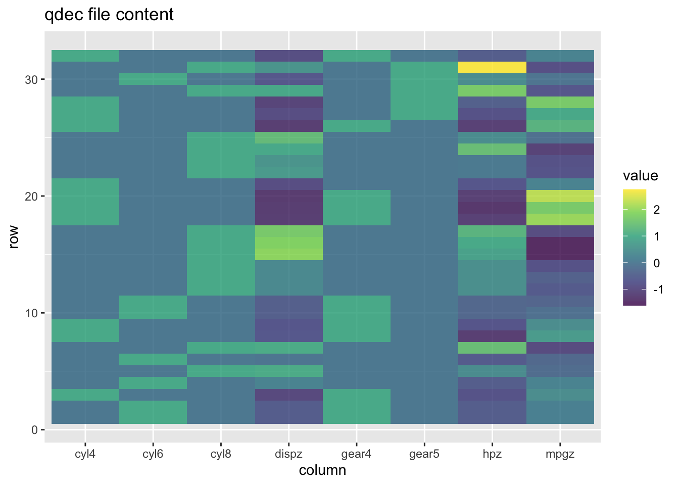
qdec |>
  mutate(row = row_number()) |>
  pivot_longer(-row, names_to = "column") |>
  ggplot(aes(y = row, x = column, fill = value)) +
  geom_tile() +
  scale_fill_viridis_c(alpha = 0.8) +
  labs(
    title = "qdec file content"
  )
Through this plot I can see which data is binary (column only has two colours), and which are continuous (column has a gradient of colours). It’s a nice way to verify that my file contains what I am after.
Mo, this is too much, I just want to use it!
Ok, I get it. You’re not here to do all the hard-coding, you just need an easy use. We all battle the balance between time spent learning to do something, and getting things done. There’s already so much to learn when doing neuroimaging, learning to write R functions for things like this is much.
I have two solutions:
- Copy paste my last function and use that
- Give my mini-package, neuromat a try
It’s the tiniest package I ever made, but it’s a package, and I hope it can ease your vertex-wise Freesurfer LMM journey! You can install it from my team’s R-Universe with:
# Install from Capro R-universe
install.packages('neuromat',
                 repos = 'https://capro-uio.r-universe.dev')
and you can have a look at the currently very minimal docs online.
rm(make_qdec, scale_vec)
library(neuromat)

make_fs_qdec(
  cars,
  mpg ~ -1 +  cyl + hp + disp + gear,
  # Keep original data columns, for comparison
  keep = c("mpg", "cyl", "hp", "disp", "gear")
)
##   cyl4 cyl6 cyl8 gear4 gear5      mpgz        hpz      dispz  mpg cyl  hp disp
## 1    0    1    0     1     0 0.1508848 -0.5350928 -0.5706198 21.0   6 110  160
## 2    0    1    0     1     0 0.1508848 -0.5350928 -0.5706198 21.0   6 110  160
## 3    1    0    0     1     0 0.4495434 -0.7830405 -0.9901821 22.8   4  93  108
##   gear
## 1    4
## 2    4
## 3    4
##  [ reached 'max' / getOption("max.print") -- omitted 29 rows ]
I hope you find it useful, and if you have any feedback, please let me know!
2024-setting-up-a-freesurfer-lmm-through-r,
author = "Dr. Mowinckel",
title = "Setting up a Freesurfer LMM through R",
url = "https://drmowinckels.io/blog/2024/freesurfer-lmm-r/",
year = 2024,
doi = "https://www.doi.org/10.5281/zenodo.13273543",
updated = "Apr 1, 2026"
}